Machine learning can feel intimidating, but at its core it starts with something surprisingly simple: the perceptron. It’s the oldest and most basic building block of neural networks, and building one from scratch is the best way to understand what’s actually happening under the hood.
In this post we’ll build a perceptron in C#, train it on the famous Iris dataset, and understand every line along the way.
The Algorithm — Before Any Code
The basic idea
Imagine you’re trying to teach a friend to tell apart apples and oranges, but they can only feel the fruit — not see it. You let them feel the weight and the texture, and each time they guess wrong, you say “warmer” or “colder” and they adjust their judgment slightly.
That’s exactly what a perceptron does. It looks at numbers (the measurements), makes a guess, gets told whether it was right or wrong, and nudges itself to do better next time.
What “learning” actually means
The perceptron has two things it can adjust:
- Weights — one number per input feature. A high weight means “this feature matters a lot”. A weight close to zero means “this feature barely matters”.
- Bias — a single extra number that shifts the decision up or down, independent of the inputs.
At the start, weights are random small numbers. The perceptron has no idea what it’s doing. After seeing enough examples and correcting itself each time, the weights settle into values that produce the right answer.
The three steps it repeats
For every example in the training data, the perceptron does exactly three things:
1. Make a prediction
Multiply each input by its weight, add them all up, add the bias. If the total is 0 or above, predict class 1. If below zero, predict class 0.
prediction = (input₁ × weight₁) + (input₂ × weight₂) + bias ≥ 0 ? → 1 : 0
2. Calculate the error
Compare the prediction to the correct answer:
error = correct answer - prediction
If the prediction was right, error = 0 and nothing changes. If it predicted 0 but the answer was 1, error = +1 → weights need to go up. If it predicted 1 but the answer was 0, error = -1 → weights need to come down.
3. Update the weights
new weight = old weight + (learning rate × error × input)
new bias   = old bias   + (learning rate × error)
The learning rate is a small number (like 0.1) that controls how aggressively it corrects itself. Too large and it overcorrects and oscillates. Too small and it learns very slowly.
Notice that inputs with larger values cause larger weight updates. If one feature is always tiny, it won’t influence the weights much. This is intentional, big inputs carry more signal.
A concrete example
Say we have one flower with sepal length 5.1 and petal length 1.4, and it’s a Setosa (correct answer = 0).
- Current weights:
[0.02, -0.01], bias:0.0 - Net input:
(5.1 × 0.02) + (1.4 × -0.01) + 0.0 = 0.102 - 0.014 = 0.088 - Prediction:
0.088 ≥ 0→ predict 1 - Error:
0 - 1 = -1(wrong — should have been 0) - Update with learning rate 0.1:
weight₁ = 0.02 + (0.1 × -1 × 5.1) = 0.02 - 0.51 = -0.49weight₂ = -0.01 + (0.1 × -1 × 1.4) = -0.01 - 0.14 = -0.15bias = 0.0 + (0.1 × -1) = -0.1
Next time it sees this flower, the lower weights will produce a lower net input, making it less likely to predict 1. Over many examples it finds the right balance.
When does it stop learning?
Either after a fixed number of passes through the data (epochs), or when it makes zero mistakes on a full pass, meaning it has found weights that correctly classify every example.
This is only guaranteed to happen if the two classes can be separated by a straight line. If they can’t, the perceptron will never settle, it will keep adjusting forever. That limitation is what led to the invention of multi-layer neural networks.
What is a Perceptron?
A perceptron is a binary classifier, it looks at some input numbers and decides: is this thing in group A or group B?
Think of it like a light switch with a dimmer. You feed it some numbers, it adds them all up (with some weights applied), and if the total is high enough, the switch flips on (class 1). If not, it stays off (class 0).
input 1 × weight 1 ┐
input 2 × weight 2 ├──→ sum + bias ──→ is it ≥ 0? ──→ yes=1 / no=0
input 3 × weight 3 ┘
The clever part: if it gets the answer wrong, it adjusts the weights slightly so it does better next time. Do this enough times and it learns to classify correctly.
The Dataset
We’ll use the Iris dataset, a classic. It contains measurements of 150 iris flowers across three species. We’ll only use two species (Setosa and Versicolor) to keep it a binary problem, and two features: sepal length and petal length.
Let’s load it directly from the UCI repository:
static async Task<(double[][] X, int[] y)> LoadIrisAsync()
{
    const string url = "https://archive.ics.uci.edu/ml/machine-learning-databases/iris/iris.data";
    using var client = new HttpClient();
    string csv = await client.GetStringAsync(url);

    var X = new List<double[]>();
    var y = new List<int>();

    foreach (var line in csv.Split('\n'))
    {
        var parts = line.Trim().Split(',');
        if (parts.Length < 5) continue;

        string label = parts[4];
        if (label != "Iris-setosa" && label != "Iris-versicolor") continue;

        // sepal length (col 0) and petal length (col 2)
        X.Add([double.Parse(parts[0]), double.Parse(parts[2])]);
        y.Add(label == "Iris-setosa" ? 0 : 1);
    }

    return (X.ToArray(), y.ToArray());
}
X is our feature matrix, each row is one flower, each column is one measurement. y is our label array — 0 for Setosa, 1 for Versicolor.
The Perceptron Class
public class Perceptron(double eta = 0.01, int epochs = 50, int randomState = 1)
Three parameters:
eta(learning rate) — how big a step the perceptron takes when it adjusts weights. Too high and it overshoots; too low and it learns painfully slowly.epochs— how many full passes through the training data.randomState— a seed for the random number generator so results are reproducible.
Step 1: Initialise the Weights
Weights = new double[X[0].Length];
for (int i = 0; i < Weights.Length; i++)
    Weights[i] = NextGaussian(rng, mean: 0.0, stdDev: 0.01);

Bias = 0.0;
We start with tiny random weights (very close to zero) rather than all zeros. If everything started at zero, every weight would update by exactly the same amount each step and they’d never diverge — the perceptron would never learn different things from different features.
Bias is an extra number added to the sum that lets the decision boundary shift away from the origin.
Step 2: Train (the Fit loop)
for (int _ = 0; _ < epochs; _++)
{
    int errors = 0;
    for (int i = 0; i < X.Length; i++)
    {
        double update = eta * (y[i] - Predict(X[i]));
        for (int j = 0; j < Weights.Length; j++)
            Weights[j] += update * X[i][j];
        Bias += update;
        if (update != 0.0) errors++;
    }
    ErrorsPerEpoch.Add(errors);
}
For each flower in the training data:
- Make a prediction — does it think this is Setosa (0) or Versicolor (1)?
- Calculate the error —
target - prediction. If it was right, this is 0. If wrong, it’s either +1 or -1. - Adjust the weights — multiply the error by the learning rate and by each input feature, then add that to the weight. Features that were large get a bigger nudge.
- Adjust the bias — same idea, just without the feature multiplication.
If update is 0 the prediction was correct and nothing changes. The perceptron only learns from its mistakes.
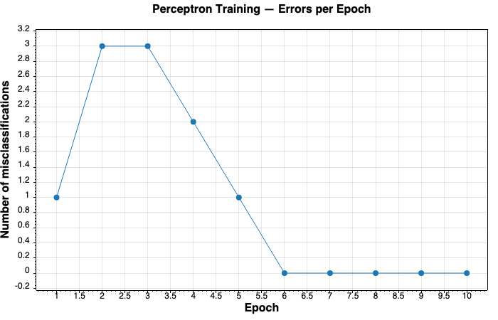
After each epoch we record how many mistakes were made (ErrorsPerEpoch). A well-trained perceptron will show this number trending down toward zero.
Step 3: Predict
public double NetInput(double[] X)
{
    double result = Bias;
    for (int i = 0; i < Weights.Length; i++)
        result += X[i] * Weights[i];
    return result;
}

public int Predict(double[] X) => NetInput(X) >= 0.0 ? 1 : 0;
NetInput is the weighted sum: multiply each feature by its weight, add the bias, and return the total.
Predict applies the unit step function: if the sum is 0 or above, predict class 1; otherwise predict class 0. That’s the threshold the perceptron uses to make its decision.
Putting it all together
var (X, y) = await LoadIrisAsync();

var ppn = new Perceptron(eta: 0.1, epochs: 10, randomState: 42);
ppn.Fit(X, y);

Console.WriteLine("Weights: " + string.Join(", ", ppn.Weights.Select(w => w.ToString("F4"))));
Console.WriteLine("Bias: " + ppn.Bias);
Console.WriteLine("Errors per epoch: " + string.Join(", ", ppn.ErrorsPerEpoch));
Console.WriteLine("Prediction for [5.1, 1.4]: " + ppn.Predict([5.1, 1.4]));
Run this and you’ll see something like:
Loaded 100 samples from UCI
Weights: -0.3715, 0.9307
Bias: -0.2
Errors per epoch: 1, 3, 3, 2, 1, 0, 0, 0, 0, 0
Prediction for [5.1, 1.4]: 0
The errors start at 1, climb slightly as the weights adjust, then settle to zero by epoch 6, the perceptron has learned to correctly separate the two flower species. The prediction of 0 for [5.1, 1.4] is correct — that’s a Setosa flower.
Why Does This Work?
The two flower species happen to be linearly separable: if you plot them on a graph by sepal length and petal length, you can draw a straight line that separates them cleanly. The perceptron finds that line.
This is also the perceptron’s main limitation: if the data can’t be separated by a straight line, it will never converge. That’s what motivated the invention of multi-layer neural networks — stacking perceptrons so they can learn curved, complex boundaries.
But for linearly separable problems, the original 1958 perceptron still works perfectly.
Full Code
var (X, y) = await LoadIrisAsync();

var ppn = new Perceptron(eta: 0.1, epochs: 10, randomState: 42);
ppn.Fit(X, y);

Console.WriteLine("Weights: " + string.Join(", ", ppn.Weights.Select(w => w.ToString("F4"))));
Console.WriteLine("Bias: " + ppn.Bias);
Console.WriteLine("Errors per epoch: " + string.Join(", ", ppn.ErrorsPerEpoch));
Console.WriteLine("Prediction for [5.1, 1.4]: " + ppn.Predict([5.1, 1.4]));

static async Task<(double[][] X, int[] y)> LoadIrisAsync()
{
    const string url = "https://archive.ics.uci.edu/ml/machine-learning-databases/iris/iris.data";
    using var client = new HttpClient();
    string csv = await client.GetStringAsync(url);

    var X = new List<double[]>();
    var y = new List<int>();

    foreach (var line in csv.Split('\n'))
    {
        var parts = line.Trim().Split(',');
        if (parts.Length < 5) continue;

        string label = parts[4];
        if (label != "Iris-setosa" && label != "Iris-versicolor") continue;

        X.Add([double.Parse(parts[0]), double.Parse(parts[2])]);
        y.Add(label == "Iris-setosa" ? 0 : 1);
    }

    return (X.ToArray(), y.ToArray());
}

public class Perceptron(double eta = 0.01, int epochs = 50, int randomState = 1)
{
    public double[] Weights { get; private set; } = [];
    public double Bias { get; private set; }
    public List<int> ErrorsPerEpoch { get; private set; } = [];

    public Perceptron Fit(double[][] X, int[] y)
    {
        var rng = new Random(randomState);
        Weights = new double[X[0].Length];
        for (int i = 0; i < Weights.Length; i++)
            Weights[i] = NextGaussian(rng, mean: 0.0, stdDev: 0.01);

        Bias = 0.0;
        ErrorsPerEpoch = [];

        for (int _ = 0; _ < epochs; _++)
        {
            int errors = 0;
            for (int i = 0; i < X.Length; i++)
            {
                double update = eta * (y[i] - Predict(X[i]));
                for (int j = 0; j < Weights.Length; j++)
                    Weights[j] += update * X[i][j];
                Bias += update;
                if (update != 0.0) errors++;
            }
            ErrorsPerEpoch.Add(errors);
        }
        return this;
    }

    public double NetInput(double[] X)
    {
        double result = Bias;
        for (int i = 0; i < Weights.Length; i++)
            result += X[i] * Weights[i];
        return result;
    }

    public int Predict(double[] X) => NetInput(X) >= 0.0 ? 1 : 0;

    private static double NextGaussian(Random rng, double mean, double stdDev)
    {
        double u1 = 1.0 - rng.NextDouble();
        double u2 = 1.0 - rng.NextDouble();
        double z = Math.Sqrt(-2.0 * Math.Log(u1)) * Math.Sin(2.0 * Math.PI * u2);
        return mean + stdDev * z;
    }
}
Explore SharpLsp
SharpLsp is a modern language server built on a three-tier architecture with a Rust host for ultra-fast syntax parsing and .NET sidecars for rich semantic analysis. It supports C# and F# with features like completions, diagnostics, refactoring, semantic tokens, and project system integration. Check out the link below to try it out!!